Gensim - Developing Word Embedding
The chapter will help us understand developing word embedding in Gensim.
Word embedding, approach to represent words & document, is a dense vector representation for text where words having the same meaning have a similar representation. Following are some characteristics of word embedding −
It is a class of technique which represents the individual words as real-valued vectors in a pre-defined vector space.
This technique is often lumped into the field of DL (deep learning) because every word is mapped to one vector and the vector values are learned in the same way a NN (Neural Networks) does.
The key approach of word embedding technique is a dense distributed representation for every word.
Different Word Embedding Methods/Algorithms
As discussed above, word embedding methods/algorithms learn a real-valued vector representation from a corpus of text. This learning process can either use with the NN model on task like document classification or is an unsupervised process such as document statistics. Here we are going to discuss two methods/algorithm that can be used to learn a word embedding from text −
Word2Vec by Google
Word2Vec, developed by Tomas Mikolov, et. al. at Google in 2013, is a statistical method for efficiently learning a word embedding from text corpus. It’s actually developed as a response to make NN based training of word embedding more efficient. It has become the de facto standard for word embedding.
Word embedding by Word2Vec involves analysis of the learned vectors as well as exploration of vector math on representation of words. Following are the two different learning methods which can be used as the part of Word2Vec method −
- CBoW(Continuous Bag of Words) Model
- Continuous Skip-Gram Model
GloVe by Standford
GloVe(Global vectors for Word Representation), is an extension to the Word2Vec method. It was developed by Pennington et al. at Stanford. GloVe algorithm is a mix of both −
- Global statistics of matrix factorization techniques like LSA (Latent Semantic Analysis)
- Local context-based learning in Word2Vec.
If we talk about its working then instead of using a window to define local context, GloVe constructs an explicit word co-occurrence matrix using statistics across the whole text corpus.
Developing Word2Vec Embedding
Here, we will develop Word2Vec embedding by using Gensim. In order to work with a Word2Vec model, Gensim provides us Word2Vec class which can be imported from models.word2vec. For its implementation, word2vec requires a lot of text e.g. the entire Amazon review corpus. But here, we will apply this principle on small-in memory text.
Implementation Example
First we need to import the Word2Vec class from gensim.models as follows −
from gensim.models import Word2Vec
Next, we need to define the training data. Rather than taking big text file, we are using some sentences to implement this principal.
sentences = [
   ['this', 'is', 'gensim', 'tutorial', 'for', 'free'],
   ['this', 'is', 'the', 'tutorials' 'point', 'website'],
   ['you', 'can', 'read', 'technical','tutorials', 'for','free'],
   ['we', 'are', 'implementing','word2vec'],
   ['learn', 'full', 'gensim', 'tutorial']
]
Once the training data is provided, we need to train the model. it can be done as follows −
model = Word2Vec(sentences, min_count=1)
We can summarise the model as follows −;
print(model)
We can summarise the vocabulary as follows −
words = list(model.wv.vocab)
print(words)
Next, let’s access the vector for one word. We are doing it for the word ‘tutorial’.
print(model['tutorial'])
Next, we need to save the model −
model.save('model.bin')
Next, we need to load the model −
new_model = Word2Vec.load('model.bin')
Finally, print the saved model as follows −
print(new_model)
Complete Implementation Example
from gensim.models import Word2Vec
sentences = [
   ['this', 'is', 'gensim', 'tutorial', 'for', 'free'],
   ['this', 'is', 'the', 'tutorials' 'point', 'website'],
   ['you', 'can', 'read', 'technical','tutorials', 'for','free'],
   ['we', 'are', 'implementing','word2vec'],
   ['learn', 'full', 'gensim', 'tutorial']
]
model = Word2Vec(sentences, min_count=1)
print(model)
words = list(model.wv.vocab)
print(words)
print(model['tutorial'])
model.save('model.bin')
new_model = Word2Vec.load('model.bin')
print(new_model)
Output
Word2Vec(vocab=20, size=100, alpha=0.025)
[
   'this', 'is', 'gensim', 'tutorial', 'for', 'free', 'the', 'howcodex',
   'website', 'you', 'can', 'read', 'technical', 'tutorials', 'we', 'are',
   'implementing', 'word2vec', 'learn', 'full'
]
[
   -2.5256255e-03 -4.5352755e-03 3.9024993e-03 -4.9509313e-03
   -1.4255195e-03 -4.0217536e-03 4.9407515e-03 -3.5925603e-03
   -1.1933431e-03 -4.6682903e-03 1.5440651e-03 -1.4101702e-03
   3.5070938e-03 1.0914479e-03 2.3334436e-03 2.4452661e-03
   -2.5336299e-04 -3.9676363e-03 -8.5054158e-04 1.6443320e-03
   -4.9968651e-03 1.0974540e-03 -1.1123562e-03 1.5393364e-03
   9.8941079e-04 -1.2656028e-03 -4.4471184e-03 1.8309267e-03
   4.9302122e-03 -1.0032534e-03 4.6892050e-03 2.9563988e-03
   1.8730218e-03 1.5343715e-03 -1.2685956e-03 8.3664013e-04
   4.1721235e-03 1.9445885e-03 2.4097660e-03 3.7517555e-03
   4.9687522e-03 -1.3598346e-03 7.1032363e-04 -3.6595813e-03
   6.0000515e-04 3.0872561e-03 -3.2115565e-03 3.2270295e-03
   -2.6354722e-03 -3.4988276e-04 1.8574356e-04 -3.5757164e-03
   7.5391348e-04 -3.5205986e-03 -1.9795434e-03 -2.8321696e-03
   4.7155009e-03 -4.3349937e-04 -1.5320212e-03 2.7013756e-03
   -3.7055744e-03 -4.1658725e-03 4.8034848e-03 4.8594419e-03
   3.7129463e-03 4.2385766e-03 2.4612297e-03 5.4920948e-04
   -3.8912550e-03 -4.8226118e-03 -2.2763973e-04 4.5571579e-03
   -3.4609400e-03 2.7903817e-03 -3.2709218e-03 -1.1036445e-03
   2.1492650e-03 -3.0384419e-04 1.7709908e-03 1.8429896e-03
   -3.4038599e-03 -2.4872608e-03 2.7693063e-03 -1.6352943e-03
   1.9182395e-03 3.7772327e-03 2.2769428e-03 -4.4629495e-03
   3.3151123e-03 4.6509290e-03 -4.8521687e-03 6.7615538e-04
   3.1034781e-03 2.6369948e-05 4.1454583e-03 -3.6932561e-03
   -1.8769916e-03 -2.1958587e-04 6.3395966e-04 -2.4969708e-03
]
Word2Vec(vocab=20, size=100, alpha=0.025)
Visualising Word Embedding
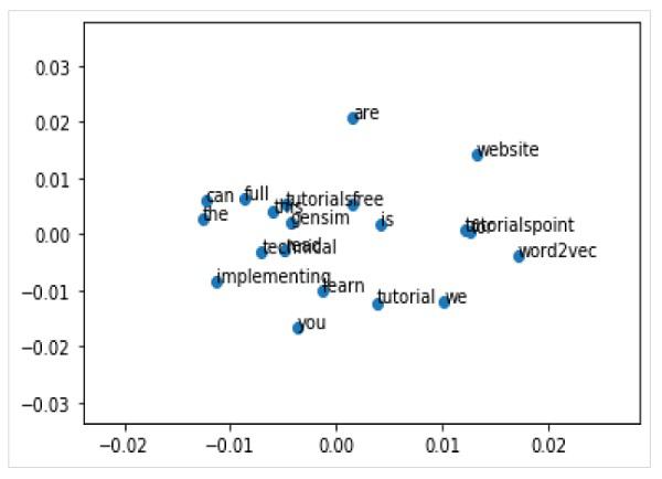
We can also explore the word embedding with visualisation. It can be done by using a classical projection method (like PCA) to reduce the high-dimensional word vectors to 2-D plots. Once reduced, we can then plot them on graph.
Plotting Word Vectors Using PCA
First, we need to retrieve all the vectors from a trained model as follows −
Z = model[model.wv.vocab]
Next, we need to create a 2-D PCA model of word vectors by using PCA class as follows −
pca = PCA(n_components=2)
result = pca.fit_transform(Z)
Now, we can plot the resulting projection by using the matplotlib as follows −
Pyplot.scatter(result[:,0],result[:,1])
We can also annotate the points on the graph with the words itself. Plot the resulting projection by using the matplotlib as follows −
words = list(model.wv.vocab)
for i, word in enumerate(words):
   pyplot.annotate(word, xy=(result[i, 0], result[i, 1]))
Complete Implementation Example
from gensim.models import Word2Vec
from sklearn.decomposition import PCA
from matplotlib import pyplot
sentences = [
   ['this', 'is', 'gensim', 'tutorial', 'for', 'free'],
	['this', 'is', 'the', 'tutorials' 'point', 'website'],
	['you', 'can', 'read', 'technical','tutorials', 'for','free'],
	['we', 'are', 'implementing','word2vec'],
	['learn', 'full', 'gensim', 'tutorial']
]
model = Word2Vec(sentences, min_count=1)
X = model[model.wv.vocab]
pca = PCA(n_components=2)
result = pca.fit_transform(X)
pyplot.scatter(result[:, 0], result[:, 1])
words = list(model.wv.vocab)
for i, word in enumerate(words):
   pyplot.annotate(word, xy=(result[i, 0], result[i, 1]))
pyplot.show()
Output


