PyTorch - Recurrent Neural Network
Recurrent neural networks is one type of deep learning-oriented algorithm which follows a sequential approach. In neural networks, we always assume that each input and output is independent of all other layers. These type of neural networks are called recurrent because they perform mathematical computations in a sequential manner completing one task after another.
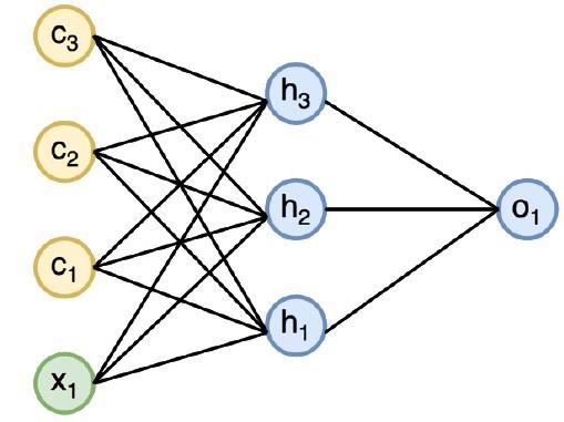
The diagram below specifies the complete approach and working of recurrent neural networks −

In the above figure, c1, c2, c3 and x1 are considered as inputs which includes some hidden input values namely h1, h2 and h3 delivering the respective output of o1. We will now focus on implementing PyTorch to create a sine wave with the help of recurrent neural networks.
During training, we will follow a training approach to our model with one data point at a time. The input sequence x consists of 20 data points, and the target sequence is considered to be same as the input sequence.
Step 1
Import the necessary packages for implementing recurrent neural networks using the below code −
import torch
from torch.autograd import Variable
import numpy as np
import pylab as pl
import torch.nn.init as init
Step 2
We will set the model hyper parameters with the size of input layer set to 7. There will be 6 context neurons and 1 input neuron for creating target sequence.
dtype = torch.FloatTensor
input_size, hidden_size, output_size = 7, 6, 1
epochs = 300
seq_length = 20
lr = 0.1
data_time_steps = np.linspace(2, 10, seq_length + 1)
data = np.sin(data_time_steps)
data.resize((seq_length + 1, 1))

x = Variable(torch.Tensor(data[:-1]).type(dtype), requires_grad=False)
y = Variable(torch.Tensor(data[1:]).type(dtype), requires_grad=False)
We will generate training data, where x is the input data sequence and y is required target sequence.
Step 3
Weights are initialized in the recurrent neural network using normal distribution with zero mean. W1 will represent acceptance of input variables and w2 will represent the output which is generated as shown below −
w1 = torch.FloatTensor(input_size,
hidden_size).type(dtype)
init.normal(w1, 0.0, 0.4)
w1 = Variable(w1, requires_grad = True)
w2 = torch.FloatTensor(hidden_size, output_size).type(dtype)
init.normal(w2, 0.0, 0.3)
w2 = Variable(w2, requires_grad = True)
Step 4
Now, it is important to create a function for feed forward which uniquely defines the neural network.
def forward(input, context_state, w1, w2):
   xh = torch.cat((input, context_state), 1)
   context_state = torch.tanh(xh.mm(w1))
   out = context_state.mm(w2)
   return (out, context_state)
Step 5
The next step is to start training procedure of recurrent neural network’s sine wave implementation. The outer loop iterates over each loop and the inner loop iterates through the element of sequence. Here, we will also compute Mean Square Error (MSE) which helps in the prediction of continuous variables.
for i in range(epochs):
   total_loss = 0
   context_state = Variable(torch.zeros((1, hidden_size)).type(dtype), requires_grad = True)
   for j in range(x.size(0)):
      input = x[j:(j+1)]
      target = y[j:(j+1)]
      (pred, context_state) = forward(input, context_state, w1, w2)
      loss = (pred - target).pow(2).sum()/2
      total_loss += loss
      loss.backward()
      w1.data -= lr * w1.grad.data
      w2.data -= lr * w2.grad.data
      w1.grad.data.zero_()
      w2.grad.data.zero_()
      context_state = Variable(context_state.data)
   if i % 10 == 0:
      print("Epoch: {} loss {}".format(i, total_loss.data[0]))

context_state = Variable(torch.zeros((1, hidden_size)).type(dtype), requires_grad = False)
predictions = []

for i in range(x.size(0)):
   input = x[i:i+1]
   (pred, context_state) = forward(input, context_state, w1, w2)
   context_state = context_state
   predictions.append(pred.data.numpy().ravel()[0])
Step 6
Now, it is time to plot the sine wave as the way it is needed.
pl.scatter(data_time_steps[:-1], x.data.numpy(), s = 90, label = "Actual")
pl.scatter(data_time_steps[1:], predictions, label = "Predicted")
pl.legend()
pl.show()
Output
The output for the above process is as follows −


