Theory of Production

In economics, production theory explains the principles in which the business has to take decisions on how much of each commodity it sells and how much it produces and also how much of raw material ie., fixed capital and labor it employs and how much it will use. It defines the relationships between the prices of the commodities and productive factors on one hand and the quantities of these commodities and productive factors that are produced on the other hand.

Concept

Production is a process of combining various inputs to produce an output for consumption. It is the act of creating output in the form of a commodity or a service which contributes to the utility of individuals.

In other words, it is a process in which the inputs are converted into outputs.

Function

The Production function signifies a technical relationship between the physical inputs and physical outputs of the firm, for a given state of the technology.

Q = f (a, b, c, . . . . . . z)

Where a,b,c ....z are various inputs such as land, labor ,capital etc. Q is the level of the output for a firm.

If labor (L) and capital (K) are only the input factors, the production function reduces to −

Q = f(L, K)

Production Function describes the technological relationship between inputs and outputs. It is a tool that analysis the qualitative input – output relationship and also represents the technology of a firm or the economy as a whole.

Production Analysis

Production analysis basically is concerned with the analysis in which the resources such as land, labor, and capital are employed to produce a firm’s final product. To produce these goods the basic inputs are classified into two divisions −

Variable Inputs

Inputs those change or are variable in the short run or long run are variable inputs.

Fixed Inputs

Inputs that remain constant in the short term are fixed inputs.

Cost Function

Cost function is defined as the relationship between the cost of the product and the output. Following is the formula for the same −

C = F [Q]

Cost function is divided into namely two types −

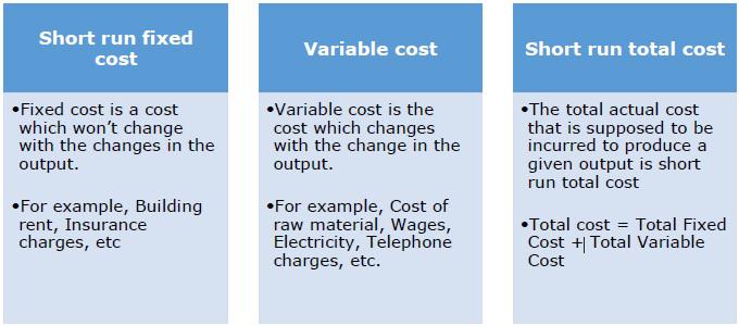
Short Run Cost

Short run cost is an analysis in which few factors are constant which won’t change during the period of analysis. The output can be changed ie., increased or decreased in the short run by changing the variable factors.

Following are the basic three types of short run cost −

Long Run Cost

Long-run cost is variable and a firm adjusts all its inputs to make sure that its cost of production is as low as possible.

Long run cost = Long run variable cost

In the long run, firms don’t have the liberty to reach equilibrium between supply and demand by altering the levels of production. They can only expand or reduce the production capacity as per the profits. In the long run, a firm can choose any amount of fixed costs it wants to make short run decisions.

Law of Variable Proportions

The law of variable proportions has following three different phases −

• Returns to a Factor
• Returns to a Scale
• Isoquants

In this section, we will learn more on each of them.

Returns to a Factor

Increasing Returns to a Factor

Increasing returns to a factor refers to the situation in which total output tends to increase at an increasing rate when more of variable factor is mixed with the fixed factor of production. In such a case, marginal product of the variable factor must be increasing. Inversely, marginal price of production must be diminishing.

Constant Returns to a Factor

Constant returns to a factor refers to the stage when increasing the application of the variable factor does not result in increasing the marginal product of the factor – rather, marginal product of the factor tends to stabilize. Accordingly, total output increases only at a constant rate.

Diminishing Returns to a Factor

Diminishing returns to a factor refers to a situation in which the total output tends to increase at a diminishing rate when more of the variable factor is combined with the fixed factor of production. In such a situation, marginal product of the variable must be diminishing. Inversely the marginal cost of production must be increasing.

Returns to a Scale

If all inputs are changed simultaneously or proportionately, then the concept of returns to scale has to be used to understand the behavior of output. The behavior of output is studied when all the factors of production are changed in the same direction and proportion. Returns to scale are classified as follows −

• Increasing returns to scale − If output increases more than proportionate to the increase in all inputs.

• Constant returns to scale − If all inputs are increased by some proportion, output will also increase by the same proportion.

• Decreasing returns to scale − If increase in output is less than proportionate to the increase in all inputs.

For example − If all factors of production are doubled and output increases by more than two times, then the situation is of increasing returns to scale. On the other hand, if output does not double even after a 100 per cent increase in input factors, we have diminishing returns to scale.

The general production function is Q = F (L, K)

Isoquants

Isoquants are a geometric representation of the production function. The same level of output can be produced by various combinations of factor inputs. The locus of all possible combinations is called the ‘Isoquant’.

Characteristics of Isoquant

• An isoquant slopes downward to the right.
• An isoquant is convex to origin.
• An isoquant is smooth and continuous.
• Two isoquants do not intersect.

Types of Isoquants

The production isoquant may assume various shapes depending on the degree of substitutability of factors.

Linear Isoquant

This type assumes perfect substitutability of factors of production. A given commodity may be produced by using only capital or only labor or by an infinite combination of K and L.

Input-Output Isoquant

This assumes strict complementarily, that is zero substitutability of the factors of production. There is only one method of production for any one commodity. The isoquant takes the shape of a right angle. This type of isoquant is called “Leontief Isoquant”.

Kinked Isoquant

This assumes limited substitutability of K and L. Generally, there are few processes for producing any one commodity. Substitutability of factors is possible only at the kinks. It is also called “activity analysis-isoquant” or “linear-programming isoquant” because it is basically used in linear programming.

Least Cost Combination of Inputs

A given level of output can be produced using many different combinations of two variable inputs. In choosing between the two resources, the saving in the resource replaced must be greater than the cost of resource added. The principle of least cost combination states that if two input factors are considered for a given output then the least cost combination will have inverse price ratio which is equal to their marginal rate of substitution.

Marginal Rate of Substitution

MRS is defined as the units of one input factor that can be substituted for a single unit of the other input factor. So MRS of x₂ for one unit of x₁ is −

Therefore the least cost combination of two inputs can be obtained by equating MRS with inverse price ratio.

x₂ * P₂ = x₁ * P₁